


Without doubt, an Excel spreadsheet is one of the most advanced tools for working with raw data—and one of the most feared. The application looks complicated, way too advanced, and like something that would take hours to figure out.
I wouldn’t be surprised if upon hearing that you had to start using MS Excel, your heart started to pound. Is there any way to make Microsoft Excel less scary and intimidating? Yes.
By learning a few spreadsheet tricks, you can bring Excel down to your level and start looking at the application in a different light. We rounded up some of the simplest yet powerful MS Excel spreadsheet tips you can start using on your data.
1. Use MS Excel Format Painter
To start you off, get yourself familiar with formatting your spreadsheet cells. A visually organized spreadsheet is highly appreciated by others as it can help them follow your data and calculations easily. To quickly apply your formatting across hundreds of cells, use the Format Painter:
- Select the cell with the formatting you wish to replicate
- Go to the Home menu and click on the Format Painter. Excel will display a paintbrush next to the cursor.
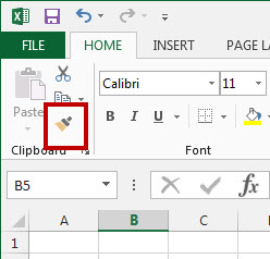 While that paintbrush is visible, click to apply all of the attributes from that cell to any other.
To format a range of cells, double-click the Format Painter during step 1. This will keep the formatting active indefinitely. Use the ESC button to deactivate it when you’re done.
2. Select Entire Spreadsheet Columns or Rows
Another quick tip– use the CTRL and SHIFT buttons to select entire rows and columns.
- Click on the first cell of the data sequence you want to select.
- Hold down CTRL + SHIFT
- Then use the arrow keys to get all the data either above, below or adjacent to the cell you’re in.
You can also use CTRL + SHIFT + * to select your entire data set.
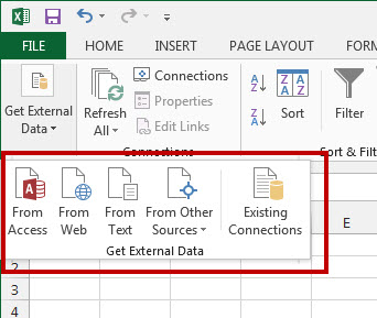
3. Import Data Into Excel Correctly
The benefit of using is Excel is that you can combine different types of data from all kinds of sources. The trick is importing that data properly so you can create Excel drop down lists or pivot tables from it.
Don’t copy-paste complex data sets. Instead, use the options from the Get External Data option under the Data tab. There are specific options for different sources. So use the appropriate option for your data:
4. Enter The Same Data Into Multiple Cells
At one point, you may find yourself needing to enter the same data into a number of different cells. Your natural instinct would be to copy-paste over and over again. But there’s a quicker way:
- Select all the cells where you need the same data filled in (use CTRL + click to select individual cells that are spread across the worksheet)
- In the very last cell you select, type in your data
- Use CTRL+ENTER. The data will be filled in for each cell you selected.
5. Display Excel Spreadsheet Formulas
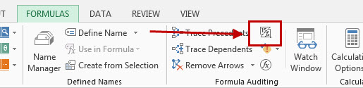
Jumping into a spreadsheet created by someone else? Don’t worry. You can easily orient yourself and find out which formulas were used. To do this, use the Show Formulas button. Or you can use CTRL + ` on your keyboard. This will give you a view of all formulas used in the workbook.
6. Freeze Excel Rows And Columns
This is a personal favourite of mine when it comes to viewing lengthy spreadsheets. Once you scroll past the first 20 rows, the first row with the column labels annoyingly disappear from view and you begin to lose track of how the data was organized.
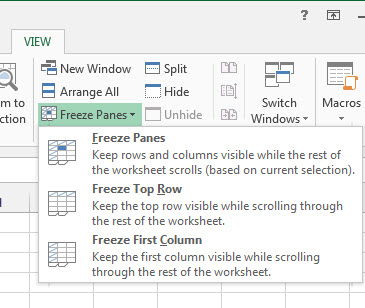
To keep them visible, use the Freeze Panes feature under the View menu. You can opt to freeze the top row or, if you have a spreadsheet with numerous columns, you can opt to freeze the first column.
7. Enter Data Patterns Instantly
One great feature in Excel is that it can automatically recognize data patterns. But what’s even better is that Excel will let you enter those data patterns to other cells.
- Simply enter your information in two cells to establish your pattern.
- Highlight the cells. There will be a small square in the bottom right hand corner of the last cell.
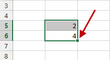
- Place your cursor over this square until it becomes a black cross.
- Then click and drag it with your mouse down to populate the cells within a column
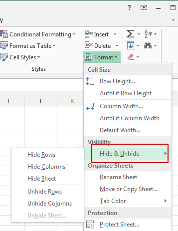
8. Hide Spreadsheet Rows and Columns
In some cases, you may have information in rows or columns that are for your eyes only and no one else’s. Isolate these cells from your work area (and prying eyes) by hiding them:
- Select the first column or row in the range you want to hide.
- Go to Format under the Home menu.
- Select Hide & Unhide>Hide Rows or Hide Columns.
To unhide them, click on the first row or column that occur just before and after the hidden range. Repeat steps 2 and 3, but select Unhide Rows or Unhide Columns.
9. Copy Formulas Or Data Between Worksheets
Another helpful tip to know is how to copy formulas and data to a separate worksheet. This is handy when you’re dealing with data that’s spread across different worksheets and requires repetitive calculations.
- With the worksheet containing the formula or data you wish to copy opened, CTRL + click on the tab of the worksheet you want to copy it to.
- Click on or navigate to the cell with the formula or data you need (in the opened worksheet).
- Press F2 to activate the cell.
- Press Enter. This will re-enter the formula or data, and it will also enter it into the same corresponding cell in the other selected worksheet as well.
These general tips won’t turn you into an Excel guru overnight. But they can help you take that first step towards becoming one! Are you a well-seasoned Excel user? Which of your spreadsheet tricks would you add?